
ROC-AUC at 0.97, Precision at 9%: The Base-Rate Math
Work through a 1%-positive detector, turn thresholds into ROC and precision-recall points, and choose an operating point for a 30-alert review budget.
Here is a detector with ROC-AUC . On a 1,000-row test set with 10 positives, its 90%-recall threshold sends 99 alerts. Nine are true. Ninety are false.
Both statements describe the same score ranking. The first rewards how well positive examples tend to rank above negative ones across all thresholds. The second describes the queue that people must actually review at one threshold. When positives are rare, those can be radically different operational stories.
This lesson builds the gap from a complete synthetic example. You will turn threshold counts into ROC and precision-recall coordinates, calculate ROC-AUC and average precision, show how prevalence moves precision without moving the ROC point, and select a threshold that fits a 30-alert review budget.
One threshold creates 99 alerts
Imagine a model that assigns a score between and to each row. The set contains 10 positives and 990 negatives, so the prevalence is
At threshold , every score at or above becomes an alert. The resulting confusion matrix is:
| Prediction | Actually positive | Actually negative | Total |
|---|---|---|---|
| Alert | TP = 9 | FP = 90 | 99 |
| No alert | FN = 1 | TN = 900 | 901 |
| Total | 10 | 990 | 1,000 |
The threshold catches nine of the ten positives. That sounds strong until the review queue is counted: 90 of its 99 alerts are false. The model has not contradicted itself. Recall and precision answer different questions.
Recall asks, “Of all actual positives, what share did the alert system catch?” Precision asks, “Of all alerts, what share were positive?” At this operating point the answers are and .
The confusion matrix supplies both coordinate systems
An ROC curve plots the true-positive rate, which is recall, against the false-positive rate:
A precision-recall curve plots precision against recall. For the threshold, the same confusion matrix gives
and . Its ROC coordinate is therefore . For the precision-recall view,
Together with recall , that becomes the precision-recall coordinate .
Now sweep six thresholds through the same ranked scores. Counts are cumulative: lowering the threshold adds both positive and negative examples to the alert set.
| Threshold | TP | FP | Alerts | Recall | FPR | Precision |
|---|---|---|---|---|---|---|
| ∞ | 0 | 0 | 0 | 0.0 | 0.0 | 1.000* |
| 0.95 | 4 | 1 | 5 | 0.4 | 0.0010 | 0.800 |
| 0.75 | 8 | 20 | 28 | 0.8 | 0.0202 | 0.286 |
| 0.55 | 9 | 90 | 99 | 0.9 | 0.0909 | 0.091 |
| 0.35 | 10 | 290 | 300 | 1.0 | 0.2929 | 0.033 |
| 0.10 | 10 | 990 | 1,000 | 1.0 | 1.0 | 0.010 |
With no predicted positives, precision is undefined. The value 1 is the conventional starting point used to draw this curve; it is not evidence of a useful classifier.
The scikit-learn precision-recall curve documentation uses the same definitions and includes endpoints for a complete curve. Its thresholds are the distinct score values; a real dataset usually supplies many more points than this compact example.
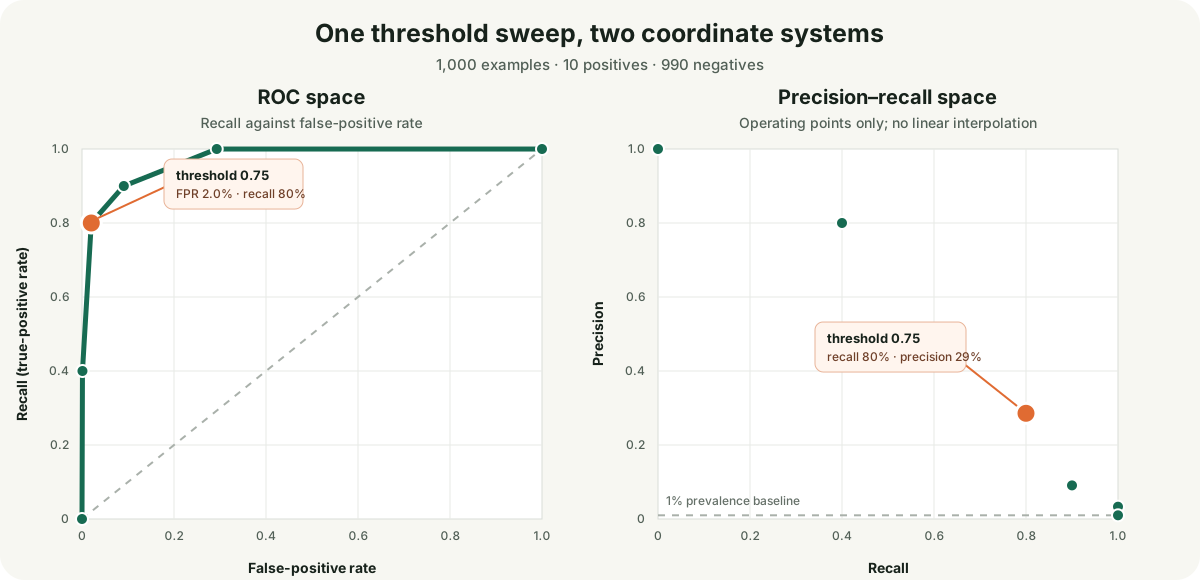
The orange point is threshold 0.75 in both panels. The coordinates change, while the underlying confusion matrix remains 8 true positives, 20 false positives, 2 false negatives, and 970 true negatives.
ROC compresses 90 false alarms into 9.1%
At threshold , the denominator of FPR contains all 990 negatives. Ninety false positives become an FPR of only . Precision instead puts the same 90 false positives beside the nine true positives that reviewers will see. That produces precision.
This is the base-rate effect in arithmetic. A small fraction of a very large negative class can outnumber most of a tiny positive class. The ROC point is valid and contains neither alert purity nor queue size.
ROC-AUC summarizes the entire ROC curve rather than any one threshold. Applying the trapezoid rule to the six points gives
scikit-learn defines ROC-AUC as the area under the ROC curve computed from prediction scores. For a binary classifier, it can also be read as the probability that a randomly selected positive receives a higher score than a randomly selected negative, with the usual handling for ties. That ranking interpretation leaves the threshold, alert count, and review cost unspecified.
The ICML 2006 analysis by Jesse Davis and Mark Goadrich shows why this distinction sharpens under class imbalance. ROC and precision-recall curves are mathematically connected for a fixed dataset, but the large negative denominator can make ROC plots look visually optimistic. They also show that straight-line interpolation in precision-recall space is generally incorrect; the curve between observed operating points is not a decorative line segment.
For this discrete sweep, non-interpolated average precision is
That is far above the precision of an uninformative ranking at this prevalence. AP still summarizes the ranking; the staffing decision requires an operating point. scikit-learn’s average-precision documentation uses the recall-weighted sum above and warns that trapezoidal interpolation can be optimistic.
Prevalence moves precision without moving the ROC point
Write prevalence as . If an operating point has true-positive rate and false-positive rate , then among a large population:
- the expected positive-alert share is ;
- the expected false-alert share is .
Precision follows by dividing the positive-alert share by all alerts:
Use the threshold, where and . Holding those conditional rates fixed gives:
| Prevalence | Expected precision |
|---|---|
| 0.1% | 3.8% |
| 1% | 28.6% |
| 10% | 81.5% |
The ROC coordinate stays near in all three rows because TPR is conditioned on positives and FPR on negatives. The precision coordinate moves dramatically because its denominator mixes true and false alerts.
This calculation assumes TPR and FPR transfer unchanged to the new population. Transfer must be tested: shifts in score distributions, labels, or data quality can move both rates. Estimate the operating point on data that represents the intended use, and keep threshold selection separate from the untouched sample used for the final performance report. The same population discipline matters when calibrating predicted probabilities.
Thirty review slots choose a threshold
Suppose the team can review at most 30 alerts per 1,000 rows and requires at least recall. The decision rule is now explicit:
The recall requirement is
Threshold fits the queue with five alerts, but its recall misses the recall requirement. Threshold creates 28 alerts and reaches recall, so it qualifies. Threshold reaches recall but creates 99 alerts, more than three times the available capacity.
The selected operating point is therefore for these rows and these constraints. Its precision is : a reviewer should expect roughly 20 false alerts among the 28, not the comfort suggested by quoting ROC-AUC alone.
Capacity can also be written as a false-positive allowance. Once the minimum number of true positives is fixed, a budget permits at most
With and eight true positives, the allowance is 22 false positives. Threshold produces 20. This translation connects model metrics to the actual resource constraint instead of assigning universal importance to one curve.
Reproduce the sweep and the budget gate
The following NumPy program calculates both curves, ROC-AUC, non-interpolated average precision, and the eligible threshold. Arrays hold cumulative counts at each descending threshold.
import numpy as np

thresholds = np.array([np.inf, 0.95, 0.75, 0.55, 0.35, 0.10])
tp = np.array([0, 4, 8, 9, 10, 10])
fp = np.array([0, 1, 20, 90, 290, 990])
positives, negatives = 10, 990

recall = tp / positives
fpr = fp / negatives
precision = np.divide(
    tp,
    tp + fp,
    out=np.ones_like(tp, dtype=float),
    where=(tp + fp) > 0,
)

roc_auc = np.trapezoid(recall, fpr)
average_precision = np.sum(np.diff(recall) * precision[1:])

budget = 30
recall_floor = 0.75
alerts = tp + fp
eligible = (alerts <= budget) & (recall >= recall_floor)

print(f"ROC-AUC: {roc_auc:.6f}")
print(f"average precision: {average_precision:.6f}")
print("eligible thresholds:", thresholds[eligible])
The output is:
ROC-AUC: 0.970808
average precision: 0.446710
eligible thresholds: [0.75]
If several thresholds qualify, choose by a declared secondary objective—such as the highest recall within budget or the lowest expected cost—not by whichever point makes a chart look best. If scores have ties, all rows at the threshold move together; a capacity target may be impossible to hit exactly.
When no threshold fits
Tighten the same budget to 25 alerts while requiring recall. Threshold catches eight positives but creates 28 alerts. The higher threshold fits the queue but catches only four positives. No row in the sweep satisfies both constraints.
That result is actionable. Moving the threshold cannot create a missing operating point. The team must improve the ranking, add a second-stage filter, increase review capacity, or accept a different recall requirement. In a real system, false positives and false negatives may also have unequal costs, so a cost function or decision analysis can replace the simple queue cap.
The broader measurement principle is current as well as mathematical. NIST AI 800-3 emphasizes that evaluators must choose a performance quantity and uncertainty method that fit the goal and data; there is no single formula for every evaluation. Here the relevant quantity is not “AUC” in the abstract. It is the recall, precision, and alert volume at a threshold for a named prevalence and a real review budget.